
Microsoft Excel (7)
Excel Tables are more than just fancy formatting. The beauty of these tables is not the instant formatting but the power it gives you in being able to analyse the data.
Since Excel 2007, you can use the Table command to convert a set of data into a formatted Excel table. Easily convert lists of data into Excel tables to easily sort, filter and view your data.
Preparing your data
Before you convert the data into a table, the data needs to be organised. Follow these guidelines to ensure your data will convert well.
- The data should be organised into rows and columns, with each row containing information about one record, such as a client, order, or expense item.
- The first row of the list should contain a short, descriptive and unique heading for each column.
- Each column in the list should contain one type of data, such as dates, currency, or text.
- Each row in the list should contain the details for one record only, like as a sales order. If possible, include a unique identifier for each row, such as an order number.
- The list should have no blank rows, and no completely blank columns.
- The list should be separated from any other data on the worksheet by at least one blank row and one blank column between the list and any other data.
When your data has been organised, you can create the formatted table. There are two ways to do this.
Convert a list into a Table
Create a table with the default table styles
- Select a single cell in the list of prepared data.
- From the Ribbon, select the Insert menu and then the Table command in the Tables grouping.
- In the Create Table dialog box, the range of your list should already be populated. Ensure that the My table has headers option is checked and adjust the range if necessary.
- Click OK to accept these settings.
You will see that the list is now automatically displayed in the default table style.
Create a table with a custom table style
- Select a single cell in the list of prepared data.
- From the Ribbon select the Format as Table button from the Home menu and then select the table style you would like to apply.
- In the Format As Table dialog box, ensure that the My table has headers option is checked and adjust the range if necessary.
- Click OK to accept these settings.
You will see that the list is now automatically displayed in the table style you selected. I like to format my tables in different colours for different lists of data and choose a sheet tab colour to match.
Let’s have a look and see what we can do now apart from admiring the pretty colours.
Rename the Table
When it is created, an Excel table is given a default name, such as Table1. I always recommend changing the name to something meaningful, so you can easily identify what the data refers to later when you are constructing formulas using this table.
- Select any cell in the table.
- From the Ribbon, select the Table Tools menu and then the Design tab. Note that the Table Tools menu only appears when a cell in the table is selected.
- At the far left of the menu, in the Properties grouping, click in the Table name box, to select the existing name.
- Type a new name without spaces, such as tblClients, and press the Enter key.
Filtering the Data
Column Filters have been automatically applied. This means you can click the dropdown arrow to the right of the column heading and apply sorting and filtering options. The option I use the most is the Search option. When I need to quickly find a record or group of records relating to a particular client or site, I type a text or number string into the search box. I can then see the related records and choose which ones I’d like to see.
Automatic totals
After you create an Excel table, it's easy to show the total for a column, or for multiple columns, using a built-in Table feature.
To show a total:
- Select any cell in the table.
- From the Ribbon, select the Table Tools menu and then the Design tab. Note that the Table Tools menu only appears when a cell in the table is selected.
- In the Table Style Options grouping, add a check the Total Row option.
- A totals row will be added at the bottom of the table, and one or more column of numbers may show a total.
To change or show other functions:
- Select the totals cell for any particular column.
- Click the dropdown arrow to the right of the selected cell.
- Select any of the listed functions or the More Functions option at the bottom of the list and proceed to add the arguments of your chosen function.
Formula Construction
You can create formulas as you would have in an ordinary list or range but you should notice that rather than a standard cell address reference, the formula references the column with structured references utilising square brackets, an @ sign, and the column name making reading your formulas much easier. For example =[@End Time]-[@Start Time]
The main benefit of a table is that formulas are automatically copied from the column when you add a new record. This helps maintain a high level of data integrity by reducing errors. You can add a new record either by inserting a new row manually or pressing the Tab key when you are in the last cell of the table (the last cell above the totals row).
When utilising totals from your table in dashboard format, you can easily read the formula because it references the table and table column names. For example =tblTasks[[#Totals],[Task Time]]. Don’t worry, if you select the cell/s you want, the names and format of the name is automatically populated, so you don’t have to type the names in.
Automatic list expansion
When you want to add a column of data to the table, all you have to do is type the new column heading in the empty cell to the right of the last column heading and press Enter.
Also read Colour your worksheet tabs
Create a button in Excel to move the user to another worksheet
It is actually fairly easy to create a button on a worksheet that you can click to take you to another sheet in the workbook. It is a fun way to get started with macros in Excel if you have never made one before.
To do this, first check that the Developer tab is visible. If not at the top with your other menus you will need to display it via the File menu. Select Options and Customize Ribbon in the left hand menu and check the Developer option in the right hand pane. Click OK to exit.
Then decide which sheet will contain the button and which sheet you will select when you click, the button. We’ll add a button to Sheet1 to take us to Sheet3.
- So click somewhere in Sheet1 and, from the Developer tab on the Ribbon, choose Record Macro.
- You need to give the macro a name that will identify later as the correct macro so in this case type GoToSheet3 in the Name box. Macro names must be all one word with no spaces.
- From the Store Macro in List choose to Store the macro in This Workbook and click OK.
Recording your macro
Excel is now in 'Record Mode' so only select the Sheet3 sheet tab click the Stop Recording button on the Developer menu.
Now we need to add a button to Sheet1 that will run the macro.
- Return to Sheet1 by selecting the Sheet1 tab and from the Developer menu, select the Insert option and click the Button (Form Control) option at the top of the drop down list. You must choose the Form Controls button and not the Active X Controls button.
- Drag the button onto the worksheet and when the Assign Macro dialog appears, click the GoToSheet3 macro and click OK.
- Select the text on the button and type Click to go to Sheet3.
- Click outside the button to deselect it and test it by clicking on the button to see it at work. When you click it you will be taken automatically to Sheet3.
If you need to make changes to the text on the button right-click on it to get access to the text. You can’t click it to select it because clicking it runs the macro attached to it.
Earlier this week I was asked a question that I’d like to share with you. The question was to do with Microsoft Excel and navigation in a workbook that has dozens of worksheets.
“Is there an easy way to get to a named tab rather than having to scroll through the many tabs going backwards and forwards?”
If you're already using the arrow buttons to the left of the sheet tabs to skip one by one or to the end and start of the sheets, you may like this quick tip.
- Hold your CTRL + left click on the arrow buttons to the left of the sheet tabs to skip to the last worksheet.
But even better than that, I hope you're going to love my favourite tip to reveal a list of your sheets.
- Right-click on the arrow buttons to the left of the sheet tabs to view a list of the sheets. Double-click to select the sheet.
If you're willing to give macros a try, you could add a button to the main worksheets so you can jump to it in a click. See this tip to walk you through how. How to Create an Excel Macro Button

When using a spread sheet program it’s easy for errors to creep in if you are not vigilant.
At this time of year when spread sheets are being used to generate End of Year results and updating for use in the new Financial Year, it’s important to check your formulae are still doing what you want and expect them to be doing.
There is an easy way to check your formulas rather than having to select each cell, giving you an easy way to scan your formulae for inconsistencies
If you are using Excel, you may not be aware that you can toggle between 'Normal View' and a 'Formula View.
- Switch views by using the CTRL +` (the one under your escape key) to reveal the formulas in your sheet. CTRL + ` to switch back to Normal View.
- Or, in the Formulas tab you can find the Show Formulas button.
Error Checking Tips
Scan your worksheet columns for visual inconsistencies and accidental overtypes.
If you select a cell, the cells utilised in the formula are highlighted.

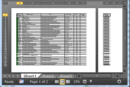
Don’t save a workbook with that annoying column stuck on page 2 or a lonely row left by itself again when you print it! Switch to Page Layout view in a single click before you adjust your column widths to ensure you only need to do it once.
The default view in Excel is Normal View. You can easily change to Page Layout view by clicking the middle button on your Status bar at the bottom of the screen, on the right, to the left of the zoom slider (highlighted in orange). The left of the Status bar also tells you how many pages your document is.
Once in Page Layout view, you can:
- Adjust your column widths. You can still double-click between the headings of the columns to automatically adjust their width to the size of the data.
- Adjust your row heights. Highlight the work sheet or rows and right-click to bring up the Shortcut Menu, then Row Height. Slightly adjust the value.
- Adjust your margins. View your ruler by selecting the View tab > Show grouping > tick Ruler.
Note: This screenshot is from Excel 2010 although all options are available in later versions.

When you have too much to fit on one page, Excel inserts automatic page breaks. As a result, information that should appear together, may be forced onto different pages. To control where the breaks appear, you can insert manual page breaks or adjust the automatic ones.
You can see the page breaks if you switch to Page Break view. Either click the Page Break Preview button to the right of the Status bar at the bottom of the screen (next to your Zoom slider); or, go to the View tab > Workbook views grouping > Page Break Preview button.

When in Page Break preview, the blue lines represent the page breaks. If you hover over the horizontal or vertical lines, your cursor will change into a double-headed arrow and you can adjust them by clicking and dragging to the appropriate location.
To add a page break:
Select the first cell you want to appear on the new page
Right-click and select Insert Page Break.
To remove a page break:
Simply click on the blue line and drag it either horizontally down off the page, or vertically off to the side.
To get back to the Normal view of the worksheet, select the Normal button to the left of the Page Break Preview button, or, go to the View tab > Workbook views grouping > Normal button.

You could go wild colour coding your worksheet tabs creating a real kaleidoscope. But if you use the colours sparingly and allocate say two different colours to your main two sheets, you won’t need to spend that extra second reading the tab names because you’ll recognise the colours more quickly and be able to switch between to sheets more quickly.
Try it:
- Right click a worksheet tab to display the shortcut menu.
- Choose Tab Colour to open the colour palette.
- Select the colour you want to apply to that tab.
- Select another tab to see the result.